The Lead Scoring Trap: When Predictive Models Learn the Wrong Patterns

The transition from biased to fair lead scoring doesn't require a complete system overhaul.

Your lead scoring model is lying to you. Not intentionally, but systematically. While you're celebrating the 90% accuracy rate and the clean ROI metrics in your quarterly review, your algorithm may be quietly learning to discriminate against entire market segments based on historical patterns that may no longer serve your business.

This isn't hyperbole.

A systematic review of 44 lead scoring studies published in Information Technology and Management found that most predictive models lack the frameworks necessary to detect bias, despite their growing adoption across industries. The problem is so widespread that Experian's research reveals 94% of organizations suspect their customer data is inaccurate, with duplicate rates reaching 10% in systems without proper data governance.

When machine learning algorithms train on this corrupted foundation, they don't just perpetuate existing biases—they amplify them at scale, making thousands of systematically flawed decisions daily while appearing mathematically objective.

The Seductive Promise That Became a Liability

Traditional lead scoring was clearly broken. Research published in Frontiers in Artificial Intelligence analysing B2B companies found that manual methods "lack formal statistical validation" and force sales reps to "spend too much time dealing with a large volume of low quality leads that will not convert into customers." These manual systems became "inaccurate, arbitrary and biased methods" that wasted resources and frustrated sales teams.

Machine learning promised to solve this. The success stories were compelling: Intelliarts documented a case study where they built a 90% accurate model for an insurance company that "cut off approximately 6% of non-efficient leads, which resulted in a 1.5% increase in profit in a few months." The highest-scoring leads converted at rates "3.5 times bigger than the average conversion." Similar wins started appearing across industries, with companies reporting dramatic improvements in sales efficiency and revenue per lead.

But these algorithms learned more than just conversion patterns.

They absorbed decades of historical decision-making, market limitations, and systematic exclusions that shaped the training data. Research on bias in credit scoring reveals how "traditional credit scoring models may inadvertently reflect and reinforce historical prejudices, leading to discriminatory outcomes" where "minority groups may receive lower credit scores not solely based on their financial behavior but rather due to the lack of historical data or access to credit opportunities."

The same dynamic affects lead scoring. A sales team that historically focused on large enterprise accounts trains an algorithm that systematically undervalues prospects from emerging companies. A model trained on data from a company with geographic limitations continues to score leads from new markets poorly, even when expansion into those regions becomes strategically important.

When Data Quality Becomes a Discrimination Engine

The foundation of every biased lead scoring model is corrupted data, and the corruption runs deeper than most teams realise. Studies on lead scoring data quality identify multiple failure modes that compound into systematic bias.

Duplicate records create the most obvious problems. When the same prospect appears multiple times in your CRM with different scores, the algorithm learns inconsistent patterns about what makes prospects valuable. But the deeper issue is selection bias in historical data. If your sales team historically avoided certain types of prospects due to resource constraints or market focus, your training data systematically underrepresents those segments. The algorithm interprets this absence as evidence that these prospects are less valuable, creating a self-reinforcing cycle of exclusion.

Geographic bias emerges when historical sales data reflects operational limitations rather than market potential. A company that sold primarily on the East Coast due to sales team distribution will train models that systematically undervalue West Coast prospects, even if market conditions have changed. Research on machine learning bias patterns documents how "an algorithm that was trained on historical hiring data that contain biases against women or minorities may perpetuate these biases in its hiring recommendations."

Temporal bias creates another layer of complexity. Customer behaviour, market conditions, and competitive landscapes evolve faster than most retraining cycles. Analysis of model drift warns that "the performance of the model you have trained on historical data can quickly deteriorate as your historical data becomes prehistorical. Our customers, market conditions, and all the features building the model are constantly changing."

The Three Failure Modes That Kill Model Performance

Data Drift: When Your Inputs Change Without Warning

Data drift occurs when the characteristics of incoming leads shift from your training data patterns. IBM's research on model drift found that "the accuracy of an AI model can degrade within days of deployment because production data diverges from the model's training data."

This manifests in subtle but destructive ways. Lead sources diversify as marketing channels evolve—social media generates different prospect profiles than trade shows. Product positioning changes affect which customer segments engage with your content. Economic conditions shift the demographics of active buyers. Your model, trained on historical patterns, begins scoring new types of qualified prospects as low-value leads.

Medical ML research provides a stark example: "when they trained and tested with data from the same OTC scanner type, they observed an overall error rate for referral of 5.5%. When the same model was used on test data acquired with a different type of OTC scanner, performance fell substantially resulting in an error rate of 46.6%." The parallel in lead scoring is a model trained on trade show leads systematically failing when applied to social media prospects.

Concept Drift: When Success Criteria Evolve

Concept drift happens when the relationship between lead characteristics and conversion probability changes over time. The features that predicted success six months ago may no longer correlate with actual conversions. Research on concept drift in machine learning explains that this occurs when "the relationships between input and output data can change over time, meaning that in turn there are changes to the unknown underlying mapping function."

Consider a B2B software company that historically sold to IT directors at large enterprises. As digital transformation accelerates, purchasing decisions migrate to business unit leaders at mid-market companies. The historical correlation between "IT Director" job titles and high conversion rates becomes obsolete, but the model continues to prioritise these prospects while undervaluing the new buyer personas driving actual revenue.

Selection Bias: Learning from Incomplete Pictures

Selection bias corrupts models when training data reflects operational constraints rather than market realities. Analysis of ML bias mitigation explains that "if a bank is developing a credit risk model using historical data on loan applications. If the bank only uses data on approved loan applications, this could result in selection bias because the data would not include information on rejected loan applications."

In lead scoring, this translates to models trained only on leads that sales teams chose to pursue, missing information about prospects that were ignored or deprioritised. The algorithm learns that certain characteristics predict conversion without understanding that these characteristics actually predicted sales attention, not inherent prospect value.

The Compounding Cost of Systematic Exclusion

These biases don't just reduce model accuracy—they systematically exclude market opportunities while appearing to optimise performance. Research on automating lead scoring documented how biased approaches lead to "waste of resources, inaccurate sales forecasts and lost sales" due to "arbitrary decisions, based on intuition when selecting leads to work with."

The business impact compounds over time. Marketing campaigns optimise toward historically successful segments, reinforcing existing biases in new data. Sales territories and hiring decisions reflect model recommendations, further embedding discrimination into operational processes. Revenue forecasts based on biased scoring models systematically underestimate potential from excluded segments.

IBM's research on AI bias warns that "when AI bias goes unaddressed, it can impact an organisation's success and hinder people's ability to participate in the economy and society." In lead scoring, this manifests as entire market segments being systematically undervalued, limiting company growth and reducing competitive positioning in emerging opportunities.

Building Bias-Resistant Lead Scoring Systems

The solution requires systematic intervention at every stage of model development and deployment. Organisations that have successfully addressed these challenges follow a consistent pattern of proactive bias detection and mitigation.

Successful implementations start with comprehensive data auditing. The ultimate checklist for accurate lead scoring emphasises that "biased data can perpetuate discrimination and inequalities in lead scoring. If data is skewed towards a particular demographic or excludes certain groups, it can result in biased predictions."

Carson Group's ML implementation achieved "96% accuracy in predicting conversion chances" by establishing robust data governance. Their success required years of historical data, multiple validation frameworks, and continuous monitoring to ensure model performance across different customer segments.

Data cleaning goes beyond deduplication. Organisations must identify and correct systematic gaps in historical data, supplement missing segments through targeted data collection, and establish ongoing validation processes that catch quality degradation before it affects model performance.

Model Development: Fairness by Design, Not by Accident

Bias mitigation must also be embedded in the modeling process, not retrofitted afterward. MATLAB's bias mitigation research demonstrates that "reweighting essentially reweights observations within a data set to guarantee fairness between different subgroups within a sensitive attribute."

Progressive Insurance's approach leveraged massive data advantages—"their Snapshot® program. Since 2008, it's collected data on over 10 billion miles of driving"—to build models that avoid demographic bias while maintaining predictive accuracy. Their success came from designing fairness constraints into the model architecture rather than trying to correct bias after training.

Cross-validation techniques prevent overfitting to biased patterns. Machine learning lead scoring best practices require "k-fold cross-validation" where "the original sample is randomly partitioned into k equal-size subsamples" to ensure "the model's value proposition is robust across different data segments."

Production Monitoring: Continuous Vigilance Against Drift

Model performance degrades inevitably in production environments. IBM's drift detection framework recommends that organisations "use an AI drift detector and monitoring tools that automatically detect when a model's accuracy decreases (or drifts) below a preset threshold."

Grammarly's Einstein Lead Scoring implementation resulted in "increased conversion rates between marketing and sales leads" by focusing on "quality over quantity" and building "trust between the two teams" through transparent monitoring and regular model updates.

Effective monitoring tracks multiple dimensions simultaneously: overall accuracy, performance across demographic segments, fairness metrics like statistical parity, and business impact measures like revenue per lead. Research on early concept drift detection introduces methods that "can detect drift even when error rates remain stable" using "prediction uncertainty index as a superior alternative to the error rate for drift detection."

Organisational Integration

Technical solutions must be supported by organisational processes that sustain bias-resistant practices. Brookings research on bias detection found that "formal and regular auditing of algorithms to check for bias is another best practice for detecting and mitigating bias."

NineTwoThree's insurance case study achieved "over 90% accuracy" through "comprehensive data collection from multiple sources" and "regular model validation and retraining." Their success required cross-functional collaboration between data science, sales, marketing, and compliance teams.

Regular algorithmic auditing becomes essential as regulatory requirements expand. The FCA's bias literature review signals that "technical methods for identifying and mitigating such biases should be supplemented by careful consideration of context and human review processes."

The ROI of Ethical AI

Organisations that proactively address bias achieve measurable competitive advantages. Lead scoring case studies demonstrate that companies implementing proper bias detection achieve "22% revenue growth in six months by fostering close cooperation between marketing and sales teams."

The cost of inaction continues rising. Regulatory frameworks are expanding rapidly, with requirements for algorithmic transparency and fairness becoming standard across industries. Companies that build bias-resistant systems today avoid compliance costs while capturing market opportunities that biased competitors systematically miss.

Research on predictive lead scoring best practices emphasises that "lead enrichment data is crucial for predictive lead scoring because it enhances models' accuracy and depth of understanding about leads" while requiring "responsibly sourced consumer data." Organisations that establish these practices early gain sustainable advantages over competitors still relying on biased legacy systems.

The choice facing practitioners is straightforward: proactively build fair, accurate lead scoring systems that capture full market potential, or reactively address bias issues while competitors dominate the segments your models systematically excluded. The research is clear, the tools are available, and the business case is compelling. The question is whether your organisation will lead or follow in the transition to bias-resistant predictive modeling.

Actionable Framework: What You Can Do Today

The transition from biased to fair lead scoring doesn't require a complete system overhaul. Practitioners can implement bias detection and mitigation strategies incrementally, starting with immediate audit steps and building toward comprehensive bias-resistant architecture.

Analyse Your Historical Conversion Data by Segment

Run this SQL query against your CRM data to identify potential bias patterns:

-- Bias Detection Query (Verified)
SELECT 
    COALESCE(lead_source, 'Unknown') as lead_source,
    COALESCE(company_size_category, 'Unknown') as company_size_category,
    COALESCE(industry, 'Unknown') as industry,
    COALESCE(geographic_region, 'Unknown') as geographic_region,
    COUNT(*) as total_leads,
    ROUND(AVG(CASE WHEN status = 'converted' THEN 1.0 ELSE 0.0 END), 4) as conversion_rate,
    ROUND(AVG(COALESCE(lead_score, 0)), 2) as avg_lead_score,
    -- Add statistical significance indicator
    CASE WHEN COUNT(*) >= 100 THEN 'Significant' ELSE 'Low Sample' END as sample_size_flag
FROM leads 
WHERE created_date >= CURRENT_DATE - INTERVAL '12 months'
    AND status IN ('converted', 'lost', 'disqualified')  -- Only include closed leads
GROUP BY 1, 2, 3, 4
HAVING COUNT(*) >= 30  -- Minimum for statistical relevance
ORDER BY conversion_rate DESC, total_leads DESC;

Look for segments with high conversion rates but low average lead scores, or segments with systematically low scores despite reasonable conversion performance.

These gaps indicate potential bias in your current model.

Calculate Statistical Parity Metrics

Research on fairness in credit scoring shows that "statistical parity difference of all subgroups" must be monitored.

Calculate this for your key demographic segments: You can use this python environment or use Replit to host one and just run the script.

import pandas as pd
import numpy as np

def calculate_statistical_parity(df, protected_attribute, prediction_column):
    """
    Calculate statistical parity difference across groups
    
    Statistical Parity Difference (SPD) = max(P(Y=1|A=a)) - min(P(Y=1|A=a))
    Where Y is the prediction and A is the protected attribute
    
    Returns SPD between 0 and 1, where 0 = perfect parity
    """
    if protected_attribute not in df.columns:
        raise ValueError(f"Protected attribute '{protected_attribute}' not found in data")
    if prediction_column not in df.columns:
        raise ValueError(f"Prediction column '{prediction_column}' not found in data")
    
    # Remove rows with missing values
    clean_df = df[[protected_attribute, prediction_column]].dropna()
    
    if len(clean_df) == 0:
        raise ValueError("No valid data after removing missing values")
    
    # Calculate rates by group
    group_rates = clean_df.groupby(protected_attribute)[prediction_column].agg(['mean', 'count'])
    
    # Filter groups with sufficient sample size
    significant_groups = group_rates[group_rates['count'] >= 10]
    
    if len(significant_groups) < 2:
        return {
            'statistical_parity_difference': None,
            'rates_by_group': group_rates['mean'],
            'bias_threshold_exceeded': False,
            'warning': 'Insufficient sample sizes for bias analysis'
        }
    
    max_rate = significant_groups['mean'].max()
    min_rate = significant_groups['mean'].min()
    spd = max_rate - min_rate
    
    return {
        'statistical_parity_difference': round(spd, 4),
        'rates_by_group': group_rates['mean'],
        'sample_sizes': group_rates['count'],
        'bias_threshold_exceeded': spd > 0.1,  # 10% threshold from research
        'severity': 'High' if spd > 0.2 else 'Medium' if spd > 0.1 else 'Low'
    }

Measure your model drift

Data drift detection is a core aspect of data observability, which is the practice of continually monitoring the quality and reliability of data flowing through an organization. The Python coding language is especially popular in data science for use in the creation of open source drift detectors.

Kolmogorov-Smirnov (K-S) test

The Kolmogorov-Smirnov (K-S) test measures whether two data sets originate from the same distribution. In the field of data science, the K-S test is nonparametric, which means that it does not require the distribution to meet any preestablished assumptions or criteria.

Data scientists use the Kolmogorov-Smirnov test for two primary reasons:

• To determine whether a data sample comes from a certain population.

• To compare two data samples and see whether they originate from the same population.

If the results of the K-S test show that two data sets appear to come from different populations, then data drift has likely occurred, making the K-S test a reliable drift detector.

Population stability index

The population stability index (PSI) compares the distribution of a categorical feature across two data sets to determine the degree to which the distribution has changed over time.

A larger divergence in distribution, represented by a higher PSI value, indicates the presence of model drift. PSI can evaluate both independent and dependent features; those which change based on other variables.

If the distribution of one or more categorical features returns a high PSI, the machine model is likely in need of recalibration or even rebuilding.

import pandas as pd
import numpy as np
from scipy.stats import ks_2samp, chi2_contingency, entropy
import matplotlib.pyplot as plt

# ---------- Helper Functions ----------

def psi(expected, actual, buckets=10):
    """Calculate Population Stability Index (PSI) for numeric features."""
    def scale_range(series, buckets):
        quantiles = np.linspace(0, 1, buckets+1)
        return np.unique(series.quantile(quantiles).values)

    breakpoints = scale_range(expected, buckets)
    expected_percents = np.histogram(expected, bins=breakpoints)[0] / len(expected)
    actual_percents = np.histogram(actual, bins=breakpoints)[0] / len(actual)

    # Avoid division by zero
    expected_percents = np.where(expected_percents == 0, 0.0001, expected_percents)
    actual_percents = np.where(actual_percents == 0, 0.0001, actual_percents)

    psi_value = np.sum((expected_percents - actual_percents) * np.log(expected_percents / actual_percents))
    return psi_value

def check_numerical_drift(base_col, curr_col):
    return {
        "PSI": psi(base_col, curr_col),
        "KS_Stat": ks_2samp(base_col, curr_col).statistic
    }

def check_categorical_drift(base_col, curr_col):
    contingency = pd.crosstab(index=base_col, columns="base")\
                   .join(pd.crosstab(index=curr_col, columns="curr"), how="outer").fillna(0)
    chi2, p, _, _ = chi2_contingency(contingency)
    return {"Chi2": chi2, "p_value": p}

# ---------- Drift Measurement ----------

def measure_drift(baseline_df, current_df, feature_types, score_col="lead_score"):
    results = []
    for col, ftype in feature_types.items():
        if ftype == "numeric":
            drift = check_numerical_drift(baseline_df[col], current_df[col])
        else:
            drift = check_categorical_drift(baseline_df[col], current_df[col])
        drift["feature"] = col
        drift["type"] = ftype
        results.append(drift)

    # Lead score drift
    if score_col in baseline_df and score_col in current_df:
        score_drift = check_numerical_drift(baseline_df[score_col], current_df[score_col])
        score_drift["feature"] = score_col
        score_drift["type"] = "lead_score"
        results.append(score_drift)

    return pd.DataFrame(results)

# ---------- Example Usage ----------

if __name__ == "__main__":
    # Replace with your actual baseline and current datasets
    baseline = pd.read_csv("baseline_lead_data.csv")
    current = pd.read_csv("current_lead_data.csv")

    # Define which features are numeric vs categorical
    feature_types = {
        "age": "numeric",
        "income": "numeric",
        "industry": "categorical",
        "region": "categorical"
    }

    drift_results = measure_drift(baseline, current, feature_types, score_col="lead_score")
    print(drift_results)

    # Save results
    drift_results.to_csv("drift_results.csv", index=False)

    # Simple visualization
    drift_results.set_index("feature")[["PSI", "KS_Stat"]].plot(kind="bar", figsize=(10,5))
    plt.title("Model Drift Metrics per Feature")
    plt.ylabel("Drift Value")
    plt.show()

If you can measure and analyse your data across these three test it will give you a very good background to understand the inherent biases that may be feeding your ML projection models.

It can help you create a simple template like this:

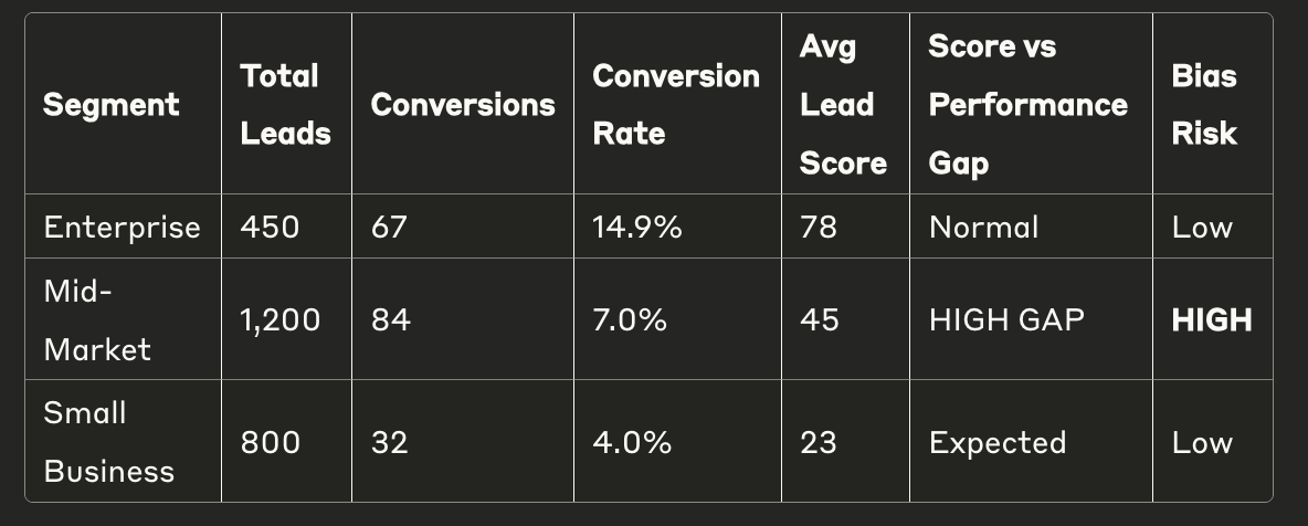
Red Flags to Look For:

• Segments with high conversion rates but low average scores

• Large gaps between predicted score and actual performance

• Systematic exclusion of profitable segments

Automation and use of ML in analysing higher value leads is necessary. But consumer buying is a very dynamic event influenced by a whole host of external and internal nuanced factors. We need to be mindful of this when we build our strategy and targeting criteria

---